This week
This week's paper, Large-scale traffic signal control using machine learning: some traffic flow considerations, caught my eye for several reasons. First, traffic signal control is relevant to my own group's work involving microservice and network traffic management. Second, the authors use cellular automaton rule 184 as their traffic model, which is actually the first time I've seen a cellular automaton used for something serious since A New Kind of Science, despite that book's claim about the likely broad usefulness of simple programs for complex purposes. Lastly, the authors find that supervised learning and random search outperform deep reinforcement learning for high-occupancies of the traffic flow network,
For occupancies > 75% during training, DRL policies perform very poorly for all traffic conditions, which means that DRL methods cannot learn under highly congested conditions.
and that they recommend practitioners throw away congested data!
Our findings imply that it is advisable for current DRL methods in the literature to discard any congested data when training, and that doing this will improve their performance under all traffic conditions.
I also have to admit that I've thought to myself, waiting at empty intersections for a light to turn green, that I could just solve this problem with DRL. If I'm wrong, that would be very interesting and surprising.
Considerations in a nutshell
The introduction and background are well summarized in their last paragraph:
In summary, most recent studies focus on developing effective and robust multi-agent DRL algorithms to achieve coordination among intersections. The number of intersections in those studies are usually limited, thus their results might not apply to large open network. Although the signal control is indeed a continuing problem, it has been always modeled as an episodic process. From the perspective of traffic considerations, expert knowledge has only been incorporated in down-scaling the size of the control problem or designing novel reward functions for DRL algorithm. Few studies have tested their methods given different traffic demands, or shed lights on the learning performance under different traffic conditions, especially the congestion regimes. To fill the gap, our study will treat the large-scale traffic control as a continuing problem and extend classical RL algorithm to fit it. More importantly, noticing the lack of traffic considerations on learning performance, we will train DRL policies under different density levels and explore the results from a traffic flow perspective.
Set up
Traffic

This is elementary cellular automaton (CA) rule 184. Elementary cellular automata operate on a binary vector, producing a new binary vector in each step that's a function of the previous one. For each entry in the previous vector, the new value of the corresponding entry in the resulting vector depends on the previous entry and its neighbors to the left and right. There are 256 possible rules with this formulation, and this picture is of the 184th rule set when ordered in the natural way.
Rule 184 can be thought of as a flow of cars along a lane of traffic. Cars move forward (right) by one cell each step only if there is an open space in front of them, otherwise they wait for one to open up. Here's an example:
def rule_184(lane):
    l = [False] + lane + [False] # pad
    return [(l[i-1] and not l[i]) or (l[i] and l[i+1])
            for i in range(1,len(l)-1)]

def show(t, lane):
    print(f't{t}:\t', ' '.join(['🚘' if i else '_' for i in lane]) )

ti = [True, True, True, True, True, False, False, True, False, False, False, False, False, False, False]

for i in range(7):
    show(i, ti)
    ti = rule_184(ti)
The cellular automaton simulates a lane of traffic, and the authors wire two of these lanes up between each adjacent traffic light to create a grid network. The network is laid out on a torus, so there are no boundaries.
The signalized network corresponds to a homogeneous grid network of bidirectional streets, with one lane per direction of length $n = 5$ cells between neighboring traffic lights.
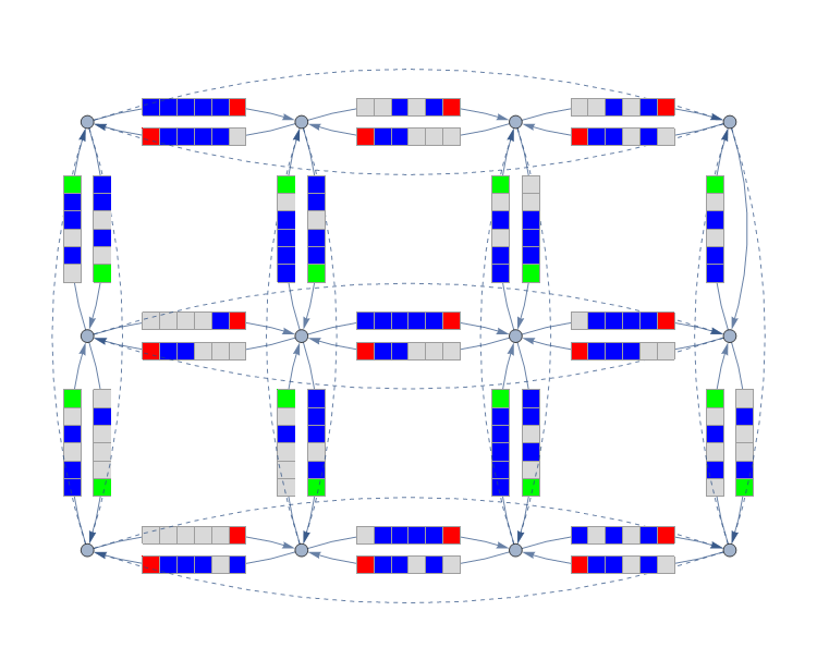
The connecting links to form the torus are shown as dashed directed links; we have omitted the cells on these links to avoid clutter. Each segment has n = 5 cells; an additional cell has been added downstream of each segment to indicate the traffic light color.
Cars arriving at a green traffic light choose a random "direction" in which to continue. Green lights are on for a minimum of three steps.
Learning
Each traffic signal is managed by an agent, which has two actions it can take at any time step: turn the light red/green for the North-South approaches, or the opposite. The state observable by each agent is an $8\times n$ matrix of bits corresponding to the four incoming and four outgoing CA vectors, and the output is the probability of turning the light red for the North-South approaches. Only one neural net is actually trained, and used by all agents, since there's no reason for them to be different in this formulation. For the DRL agent, the reward is the incremental average flow per lane (not the average flow per lane), which the authors mention is lower-variance. The authors use a custom infinite-horizon variant of REINFORCE they call REINFORCE-TD.
Experiments
The authors use a maximum-queue-first (LQF) greedy algorithm as their baseline for comparison, which services the lane with the longest queue length at all times.
Random policies
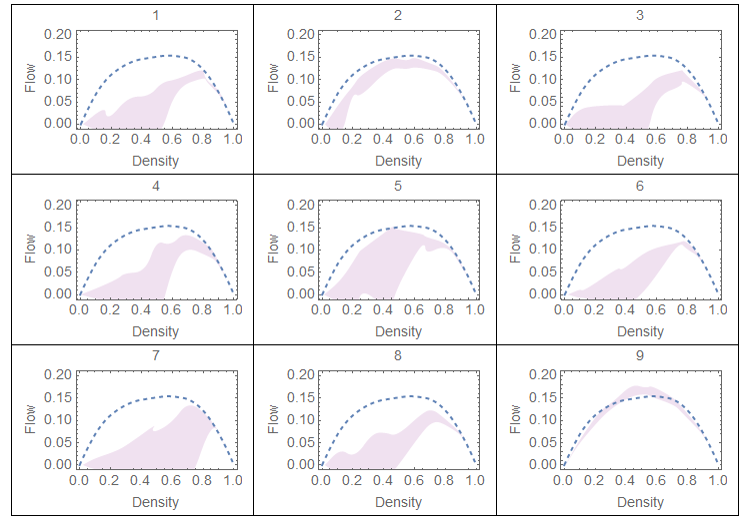
They begin by randomly reinitializing the parameters of the neural network, and discover that ~15% of random policies are competitive (that is, they can outperform LQF for some traffic densities). They also note a previously undiscovered pattern that "all policies, no matter how bad, are best when the density exceeds approximately 75%." How odd.
Supervised learning policies
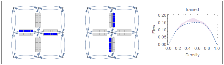
They then train a policy with supervised learning, and surprisingly, with only the two obvious extreme examples, the resulting policy is near-optimal.
DRL policies
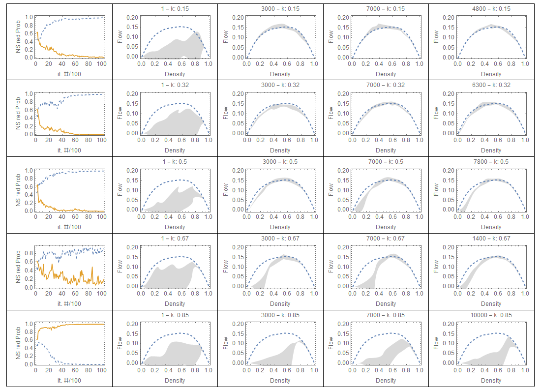
Policies trained with constant demand and random initial parameters $\theta$. The label in each diagram gives the iteration number and the constant density value. First column: NS red probabilities of the extreme states, $\pi(s1)$ in dashed line and $\pi(s2)$ in solid line. The remaining columns show the flow-density diagrams obtained at different iterations, and the last column shows the iteration producing the highest flow at $k = 0.5$, if not reported on a earlier column.
Finally, they run two experiments with DRL policies, as described above. These policies seem to do rather poorly in general compared to random search and supervised learning, and as density increases, they stop learning much of anything.
We conjecture that this result is a consequence of a property of congested urban networks and has nothing to do with the algorithm to train the DRL policy.
I'm skeptical. See my parting thoughts.
The other experiments the authors perform just confirms that average flow per lane does worse than incremental average flow per lane.
Parting thoughts
- In the end, I'm way more interested in the experimental setup of this paper than the conclusions. As usual, I learned a ton, and I may actually use rule 184 as a model for traffic flow on something.
- Isn't it obvious given their problem formulation that the agents can't learn under conditions of congestion, since it means their input is essentially whited out? I would be more impressed with the conclusion if a neural net with complete visibility had trouble learning with congestion. It also seems to me extremely suggestive that a supervised policy can learn from only two examples, and I would very much like to see if the major conclusions of this paper explode with a more realistic network topology. Queueing theory contains all sorts of counterintuitive surprises, and it seems likely to me that their results are more indicative of one of those surprises, rather than some deep fact about DRL's ability to manage urban congestion.
- It's interesting that they formulate the problem as a continuing one, against the prevailing trend in the traffic signal control literature. I agree with them, that even if you get to a state where there's no traffic, that's a function of the demand, not of the agent's choices. I bring this up because I too have found that it's really quite important to recognize an infinite-horizon problem when you have one, or else your agent learns to rack up debts until the end of the artificial episode when all is "forgiven".
- It's fascinating that all random policies, no matter how bad, are best around 75% congestion. I have been admonished to avoid scheduling myself at more than 70% capacity to avoid the ringing effect. I wonder if this is an empirical vindication of that...