Introduction
This article will dive into a lot of the math surrounding the gradients of different maximum entropy RL learning methods. Usually we work in the space of objective functions in practice: with both policy gradients and Q-learning, we'll form an objective function and allow an autodiff library to calculate the gradients for us. We never have to see what's going on behind the scenes, which has its pros and cons. A benefit is that working with objective functions is much easier than calculating gradients by hand. On the other hand, it's easy to lose sight of what's really going on when we work at such an abstract level.
This abstraction issue is tackled in the paper Equivalence Between Policy Gradients and Soft Q-Learning (https://arxiv.org/abs/1704.06440), and I think it provides some pretty eye-opening insights into what the most common RL algorithms are really doing. I'll be working off of version 4 of the paper from Oct. 2018, the most recent version of the paper at the time of writing.
First I'll walk through some of the basic definitions in the max-entropy RL setting, then I'll pick out the most important bits of math from the paper that show how entropy-augmented Q-learning is really just a policy gradient method.
Maximum Entropy RL and the Boltzmann Policy
In standard RL, we try to maximize expected cumulative reward $\mathbb{E}[\sum_t r_t]$. In the max-entropy setting, we augment this reward signal with an entropy bonus. The expected cumulative reward of a policy $\pi$ is commonly denoted as $\eta(\pi)$
\begin{align*} \eta(\pi) &= \mathbb{E} \Big[ \sum_t (r_t + \alpha \mathcal{H}(\pi)) \Big] \\ &= \mathbb{E} \Big[ \sum_t \big( r_t - \alpha \log\pi(a_t | s_t) \big) \Big] \end{align*}where $\pi$ is our current policy and $\alpha$ weights how important the entropy is in our reward definition. This intuitively makes the reward seem higher when our policy exhibits high entropy, allowing it to explore its environment more extensively. A key component of this augmented objective is that the entropy is inside the sum. Thus an optimal policy will not only try to act with high entropy now, but will act in such a way that it finds highly-entropic states in the future.
The paper uses slightly different notation, opting to use KL divergence (AKA "relative entropy") instead of just entropy. This uses a reference policy $\bar{\pi}$, which can be thought of as an old, worse policy that we wish to improve on
\begin{align*} \eta(\pi) &= \mathbb{E} \Big[ \sum_t (r_t - \alpha \log\pi(a_t|s_t) + \alpha \log\bar{\pi}(a_t|s_t) \Big] \\ &= \mathbb{E} \Big[ \sum_t \big(r_t - \alpha D_{KL}(\pi \,\Vert\, \bar{\pi}) \big) \Big] \end{align*}In the max-entropy setting, optimal policies are stochastic and proportional to exponential of the optimal Q-function. This can be expressed formally as
$$ \pi^* \propto e^{Q^*(s,a)} $$If this doesn't seem very intuitive, I would recommend a quick scan of the article https://bair.berkeley.edu/blog/2017/10/06/soft-q-learning/. It offers a brief introduction to max-entropy RL (specifically for Q-learning) and some helpful intuitions as to why the above relationship is a good property for a policy to have.
To actually get a policy in this form, we'll change up the definition slightly
$$ \pi = \frac{\bar{\pi} \, e^{Q(s,a) / \alpha}}{\mathbb{E}_{\bar{a}\sim\bar{\pi}} [e^{Q(s,\bar{a}) / \alpha}]} $$The numerator of this expression is simply stating that we want our new policy to be like our old policy, but slightly in the direction of $e^Q$. If $\alpha$ is higher (i.e. we want more entropy), we move less in the direction of $e^Q$. The denominator is a normalization constant that ensures that our entire expression is still a valid probability distribution (i.e. the sum over all possible actions comes out to 1).
You may have noticed that the denominator of our policy is really just $e^V$ since $V = \mathbb{E}_{a}[Q]$. We'll use this to simplify our policy
\begin{align*} V(s) &= \alpha \log \mathbb{E}_{a\sim\bar{\pi}} \big[ e^{Q(s,a)/\alpha} \big] \\ \pi &= \bar{\pi} \, e^{(Q(s,a) - V(s)) / \alpha} \end{align*}This new policy definition shows more directly that our policy is proportional to the exponential of the advantage. If our policy is proportional to $e^Q$, it should also be proportional to $e^A$, so this makes sense. From now on, we'll refer to this policy as the 'Boltzmann Policy' and denote it $\pi^B$.
Soft Q-Learning with Boltzmann Backups
From this point onward, there will inevitably be sections of math that seem to leave out non-trivial amounts of work. This is because I think this paper mainly benefits our intuitions about RL. The math proves these new intuitions, but by itself is hard to read. If you're curious and wish to go through all the derivations, I would highly recommend working through the full paper on your own. With that disclaimer out of the way, we can get started...
With normal Q-learning, we define our backup operator $\mathcal{T}$ as follows $$ \mathcal{T}Q = \mathbb{E}_{r,s'} \big[ r + \gamma \mathbb{E}_{a'\sim\pi}[Q(s', a')] \big] $$
In the max-entropy setting, we'll have to add in an entropy bonus to the reward signal and simplify accordingly
\begin{align*} \mathcal{T}Q &= \mathbb{E}_{r,s'} \big[ r + \gamma \mathbb{E}_{a'}[Q(s', a')] - \alpha D_{KL} \big( \pi(\cdot|s') \;\Vert\; \bar{\pi}(\cdot|s') \big) \big] \\ &= \mathbb{E}_{r,s'} \big[ r + \gamma \alpha \log \mathbb{E}_{a'\sim\bar{\pi}}[e^{Q(s',a')/\alpha}] \big] \end{align*}See equations 11 and 13 from the paper (which rely on equations 2-6) if you want to see just how exactly that simplication works. To actually perform the optimization step $Q \gets \mathcal{T}Q$, we'll minimize the mean squared error between our current $Q$ and an estimate of $\mathcal{T}Q$. Our regression targets can be defined
\begin{align*} y &= r + \gamma \alpha \log \mathbb{E}_{a'\sim\bar{\pi}} \big[ e^{Q(s', a') / \alpha} \big] \\ &= r + \gamma V(s') \end{align*}Using Boltzmann backups instead of the traditional Q-learning backups is what transforms normal Q-learning into what's conventionally called "soft" Q-learning. That's really all there is to it.
Policy Gradients and Entropy
I'm assuming you have a solid grasp of policy gradients if you're reading this article, so I'm gonna focus on how they usually aren't applied correctly in the max-entropy setting. PG methods are commonly augmented with an entropy term, like with the following example provided from the paper
$$ \mathbb{E}_{t, s,a} \Big[ \nabla_\theta \log\pi_\theta(a|s) \sum_{t' \geq t} r_{t'} - \alpha D_{KL}\big (\pi_\theta(\cdot|s) \;\Vert\; \pi(\cdot|s) \big) \Big] $$This example essentially tries to maximize reward-to-go with an entropy for the current timestep. Maximizing this objective technically isn't what we want, even if it's common practice. What we really want is to maximize a sum over all rewards and entropies that our agent experiences from now into the future.
Soft Q-Learning = Policy Gradient
The first of two conclusions that this paper comes to is that Soft Q-Learning and the Policy Gradient have exact first-order equivalence. Using the value function and Boltzmann policy definitions from earlier, we can derive the gradient of $\mathbb{E}_{s,a} \big[ \frac{1}{2} \Vert Q_\theta(s,a) - y \Vert^2 \big]$. The paper is able to produce the following expression
$$ \mathbb{E}_{s,a} \Big[ \color{red}{-\alpha \nabla_\theta \log\pi_\theta(a|s) \Delta_{TD} + \alpha^2 \nabla_\theta D_{KL}\big( \pi_\theta(\cdot|s) \;\Vert\; \bar{\pi}(\cdot|s) \big)} + \color{blue}{\nabla_\theta \frac{1}{2} \Vert V_\theta(s) - \hat{V} \Vert^2} \Big] $$where $\Delta_{TD}$ is the discounted n-step TD error and $\hat{V}$ is the value regression target formed by $\Delta_{TD}$.
That's kind of a lot, but we can break it down pretty easily. The terms in red represent 1) the usual policy gradient and 2) an additional KL divergence gradient term. The red terms overall represent the gradient you get if you use a policy gradient algorithm with a KL divergence term as your entropy bonus (the actor loss in an actor-critic formulation). The term in blue is quite simply the gradient used to minimize the mean squared error between our current value estimates and our value targets (the critic loss in an actor-critic formulation).
Don't forget that we never explicitly tried to calculate these terms. They came about naturally as an effect of minimizing mean squared error of our Q function and a Boltzmann backup target.
Soft Q-Learning and the Natural Policy Gradient
The next section of the paper details another connection between Soft Q-learning and policy gradient methods, specifically that damped Q-learning updates are exactly equivalent to natural policy gradient updates.
The natural policy gradient weights the policy gradient with the Fisher information matrix $\mathbb{E}_{s,a} \Big[ \big( \nabla_\theta \log\pi_\theta(a|s) \big)^T \big( \nabla_\theta \log\pi_\theta(a|s) \big) \Big]$. The paper shows that the natural policy gradient in the max-entropy setting is equivalent not to soft Q-learning by itself, but instead to a damped version. In this damped version, we calculate a backed-up Q value and then interpolate between it and the current Q value estimate (basically using Polyak averaging instead of running gradient descent on a mean squared error term).
Although not nearly as direct, this connection highlights how higher-order connections between soft Q-learning and policy gradient methods exist. Higher-order equalities between functions point to functions that are increasingly similar, so this connection really drives the point home that soft Q-learning is deceptively like the policy gradient methods we've been using all this time.
Experimental Results
The paper authors decided to be nice to us and actually test the theory they derived on some Atari games.
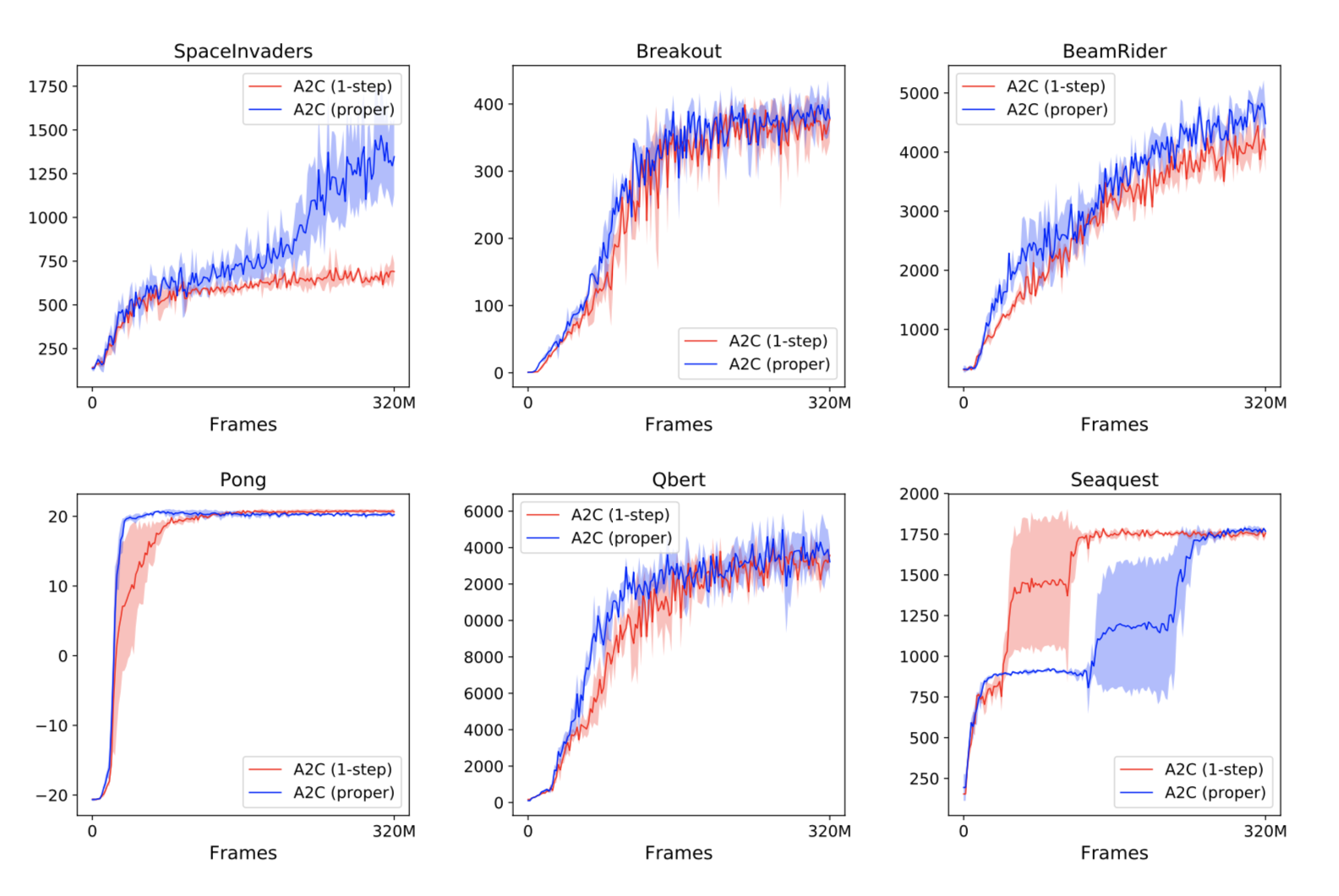
They started out with testing whether or not the usual way of adding entropy bonuses to policy gradient methods is actually worse than the theoretical claims they had just made. As it turns out, using future entropy bonuses $\Big( \text{i.e. } \big( \sum r + \mathcal{H} \big) \Big)$ instead of the simpler, immediate entropy bonus $\Big( \text{i.e. } \big( \sum r \big) + \mathcal{H} \Big)$ results in either similar or superior performance. The below graphs show the results from the experiments, with the future entropy version in blue and the immediate entropy version in red.
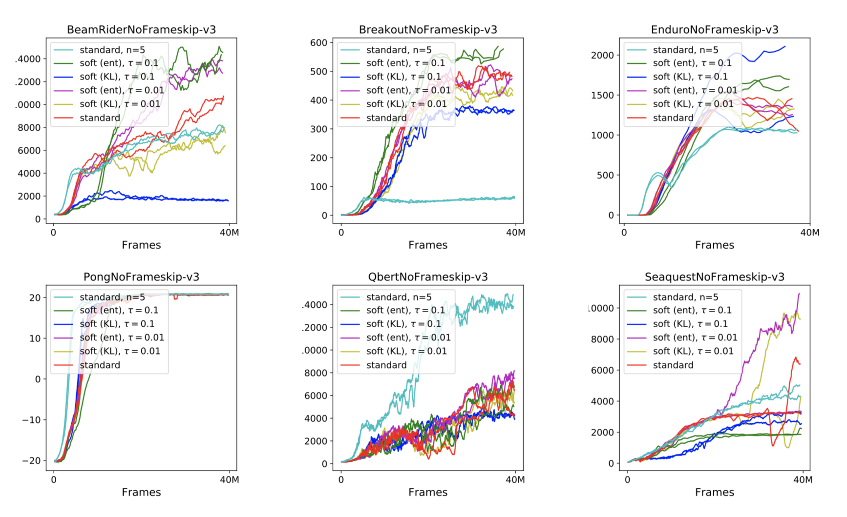
They then tested how soft Q-learning compared to normal Q-learning. To make traditional DQN into soft Q-learning, they just modified the regression targets for the Q function. They used the normal target, a target with a KL divergence penalty, and a target with just an entropy bonus. They found that just the entropy bonus resulted in the most improvement, although both soft methods outperformed the "hard" DQN.
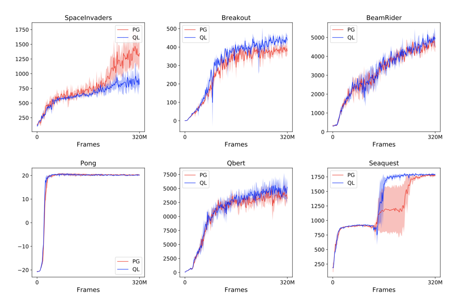
To round things out, they tested soft Q-learning and the policy gradient on the same Atari environments to see if they were equivalent in practice. After all, the math shows that their expectations are equivalent, but the variance of those expectations could be different. The experiments they ran make it seem like the two methods are pretty close to each other, with no method seeming largely superior.
Conclusion and Future Work
Hopefully this made you reconsider what's really going on under the hood with Q-learning. Personally, it blew my mind that two seemingly disparate learning methods could boil down to the same expected update. The theoretical possibilities that this connection could lead to is also incredibly exciting.
Of course, this paper focuses its empirical testing just on environemnts with discrete action spaces. Since the Boltzmann policy is intractable to sample from in continuous action spaces, more advanced soft Q-learning algorithms (such as Soft Actor-Critic) are currently being pioneered to get accurate results in those more complicated settings as well.