This week¶

This week's highlight is a paper on imitation learning: Learning Self-Correctable Policies and Value Functions from Demonstrations with Negative Sampling, chosen again for pragmatic reasons. The problem my team is currently working on has both reasons for wanting high sample efficiency: training would be prohibitively slow without something to kickstart it, and actions taken in the real world can get expensive.

I know I said I'd be experimenting with shorter, more bite-sized posts, but... next time. (If you want that, you can just stop reading after the "Key intuition" section.)

The problem¶

Learning from demonstrations is more difficult than it may seem at first glance. The trouble mainly stems from covariate shift: the input distribution your agent will see in production is very likely to be different than that encountered during training. Many machine learning algorithms have this problem, reinforcement learning algorithms included, but imitation learning has it especially bad, for a simple reason: the expert demonstrations you are attempting to follow necessarily explore a very small subset of the state space. The whole point of them is to stay on good trajectories, meaning bad trajectories never get explored.

This causes two issues:

1. The agent can't in general figure out how to get back into the subset of state space where the expert demonstrations apply, even if it gets only slightly off-course, and
2. Value functions for states and actions are affected by unseen states, making it very likely that the agent will wander off as soon as it's allowed.

Key intuition¶

The authors solve this problem by pre-training with supervised learning using a loss function that drives down the value of all states outside of those explored in the expert demonstrations $U$, by an amount proportional to their Euclidean distance from the closest state in $U$. In their own words:

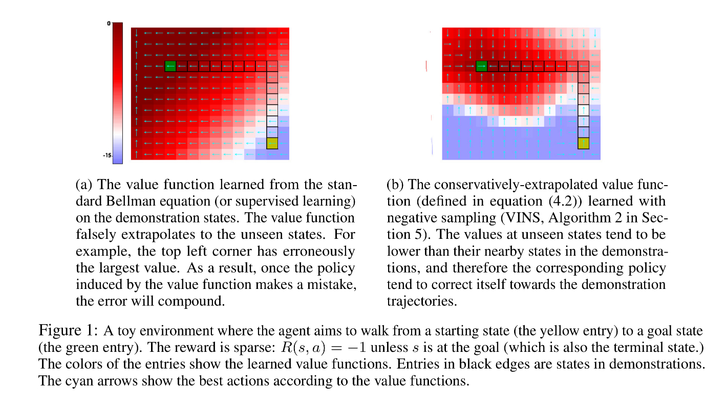
Consider a state $s$ in the demonstration and its nearby state $\tilde{s}$ that is not in the demonstration. The key intuition is that $\tilde{s}$ should have a lower value than $s$, because otherwise $\tilde{s}$ likely should have been visited by the demonstrations in the first place. If a value function has this property for most of the pair $(s,\tilde{s})$ of this type, the corresponding policy will tend to correct its errors by driving back to the demonstration states because the demonstration states have locally higher values.

And Figure 1 is a nice visual demonstration:

Value Iteration with Negative Sampling (VINS)¶

Into the weeds now.

Self-correctable policy¶

The first bit of their algorithm is the definition of their self-correcting policy. It's essentially a formalization of what we said above about $s$ and $\tilde{s}$.

If $s \in U$ (if $s$ is in the expert demonstrations), then $$V(s) = V^{\pi_e}(s) \pm \delta_V$$ ("just what the value would be in the expert demonstrations, plus some error").

But if $s \not\in U$, $$V(s) = V^{\pi_e}(\Pi_U(s)) - \lambda \|s-\Pi_U(s)\| \pm \delta_V$$ (where $\Pi_U$ gives the closest $s \in U$, so $V(s)$ is "the value of the closest $s \in U$, minus the distance to that $s \in U$, plus some error")

Then the induced policy from this value function is $$\pi(s) \triangleq \underset{a: \|a-\pi_{BC}(s)\|\le \zeta}{\operatorname{argmax}} ~V(M(s, a))$$

Where $M(s,a)$ is a learned dynamical model of the environment that gives the next state given the current state and action. $\pi_{BC}(s)$ is the "behavioral clone" policy from the expert demonstrations.

RL algorithm¶

To actually achieve $V(M(s,a))$ with the necessary properties, they select a state $s$ from the demonstrations, perturb it a bit to get $\tilde{s}$ nearby, and use the original state $s$ to approximate $\Pi_U(\tilde{s})$ in the following loss function.

$$\mathcal{L}_{ns}(\phi)= \mathbf{E}_{s \sim \rho^{\pi_e}, \tilde{s} \sim perturb(s)} \left(V_{\bar \phi}(s) - \lambda \|s-\tilde{s}\|- V_\phi(\tilde{s}) \right)^2$$

Finally, here's the algorithm that uses this and the earlier policy definition:

Parting thoughts¶

1. I thought it was quite strange that they learned $V(s)$ and a dynamical model $M(s,a)$, and then used $V(M(s,a))$ in the algorithm. I thought, "Why not just learn $Q$?" The answer was given in their Section A appendix, and was quite interesting. I'm not sure it applies to our case, but it's important. TL;DR $Q(s,a)$ learned from demonstrations alone is degenerate, because there's always a $Q$ that perfectly matches the demonstrations and doesn't depend at all on $a$.
2. One of my coworkers (and upcoming Computable author!) wondered to me if the induced policy could be made explicit, by explicitly training a policy network to bring the agent back into safe territory. It could be trained with gradient descent, because $V(M(s,a))$ are just networks, and the technique for training deterministic policies just follows the gradient of the $Q$ function. I wonder too.