It's a running joke on our team that pretty much every paper on reinforcement learning has some canned description of what RL is in their first or second section. Below is Lillicrap et al’s take on the classic formula from their paper on Deep Deterministic Policy Gradients.
We consider a standard reinforcement learning setup consisting of an agent interacting with an environment E in discrete timesteps. At each timestep $t$ the agent receives an observation $x_t$, takes an action at and receives a scalar reward $r_t$. In all the environments considered here the actions are real-valued $a_t ∈ R_N$. In general, the environment may be partially observed so that the entire history of the observation, action pairs $s_t = (x_1, a_1, ..., a_{t-1}, x_t)$ may be required to describe the state. Here, we assumed the environment is fully-observed so $s_t = x_t$. An agent’s behavior is defined by a policy, $π$, which maps states to a probability distribution over the actions $π : S → P(A)$. The environment, $E$, may also be stochastic. We model it as a Markov decision process with a state space $S$, action space $A = R_N$ , an initial state distribution $p(s1)$, transition dynamics $p(s_{1+1}|s_t, a_t)$, and reward function $r(s_t, a_t)$.
Not particularly informative for someone without a background in RL, is it? In this post I’m going to break down the various elements into chunks which will (hopefully) be easier to digest.
State
The state is a numerical representation of the environment at a given timestep, modeled as a Markov Decision Process. An MDP is a way of representing processes with discrete time steps and events that are partially random and partially controlled by a decision maker. In the context of RL, the environment may be a video game, a physical robot and its surroundings, a software system, a smart home, or any complex system we might want to manipulate. The state is technically not always the same as the observation, which is the part of the state that is observable to the agent. The two terms are often used interchangeably and in many problem spaces they refer to the same thing.When only part of the observation is observable, the environment is called a Partially Observable Markov Decision Process (POMDP). Without extra enhancements (usually RNNs), standard MDPs are much easier than POMDPs to obtain good results from.
Policy
The policy is the primary decision making mechanism in reinforcement learning. It is responsible for choosing an action to take based on the current state of the environment. In deep reinforcement learning, the policy can either be neural network or a simple max function over the values (which I elaborate upon below) of each possible action. Policies are often stochastic, meaning that they give probabilities that each possible action is the correct one and choose randomly based on those probabilities.
Reward
The reward is a single-number measure of how good or bad an agent is doing. The goal of an RL agent is to maximize the total amount of reward received. Obtaining a reward signal that is easy to learn from and highly correlated with what you want your agent to achieve can be one of the most significant challenges of applying RL. On the simpler end of the spectrum are problems like Atari games, where a consistent numerical reward (the score) can be obtained by accessing the game’s memory. A more complicated example would be a simulation in which a robotic arm must grasp an object and move it to a specific location. It would be tempting to provide a reward of 1 if the goal was achieved and 0 otherwise, however, this kind of “sparse reward signal” is extremely difficult to learn from. In practice, researchers may engineer a reward function for each task, deciding on metrics that should be encouraged or penalized because they are correlated with eventual success at the task.
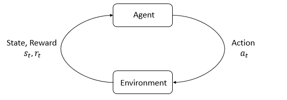
Interaction between the pieces we've covered so far. Image is from OpenAI's Spinning Up Series
Value Function
The value of a state is simply the maximum expected reward that can be obtained from that state, and the value function (is usually a neural network that) predicts the value given a state or state-action pair. In order to avoid learning extremely shortsighted behavior, value functions consider not just the immediate reward but all possible rewards that can be achieved after.
Imagine trying to learn how to perform a basic task, say, making and eating a sandwich, with total naivety and without the benefit of foresight. When faced with the choice between eating all of the bread plain or making it into a sandwich and eating that, most people would choose the latter (I hope). However, without the ability to take into account what happens in the future (eating a completed sandwich), in the moment the choice becomes one between eating the bread and not eating the bread. If eating the bread provides a reward and not eating the bread provides none, one would choose to eat the bread and never find out what happens if you postpone eating to create something else. This is the problem a value function tries to fix, by combining the predicted reward for an action with the estimated maximum possible future reward that can be obtained from a given state. In the case of the sandwich maker, eating the bread is what is called a “terminal state.” No future rewards are possible, since you have eaten all the bread and cannot make a sandwich. Not eating the bread, on the other hand, opens up the possibility of making a sandwich. While the immediate reward from this decision is zero, the value takes into account the highest possible reward that can be obtained in the future. Thus, the value takes into account the reward from eating the sandwich.
This idea is captured by the Bellman Equation, where $ Q(s, a) $ equals the value of an action $ a $ taken from a particular state $ s $ and $ r(s, a) $ equals the immediate reward for the action:
$ Q^*(s,a) = E[{r(s,a) + \gamma \max_{a'} Q^*(s',a')}] $
The equation is recursive in that $ Q(s, a) $ is defined in terms of $ Q(s’, a’) $, where $ s’ $ and $ a’ $ are the next state and action. When a terminal state is reached (the game is over), $ Q(s_{final}, a_{final}) = r $ and the recursion terminates.
Conclusion
I hope the paper quoted at the start of the post is easier to decipher now. The next post will cover classifications of environments/problems, the different types of DRL algorithms, and the trade-offs between the various approaches. In the process we will start to go into the specifics of how the abstract concepts of policy and value functions are actually implemented.